TOC Differences between DFA and NDFA

The following table lists the differences between DFA and NDFA.

DFA	NDFA
The transition from a state is to a single particular next state for each input symbol. Hence it is called deterministic.	The transition from a state can be to Multiple next states for each input symbol. Hence it is called non-deterministic.
Empty string transitions are not seen in DFA.	NDFA permits empty string transitions.
Backtracking is allowed in DFA.	In NDFA, backtracking is not always Possible
Requires more space. Requires less space. A string is accepted by a DFA, if it transits to a final state.	A string is accepted by a NDFA, if at least one of all possible transitions ends in a final state.

TOC Non-deterministic Finite Automaton (NDFA)

In NDFA, for a particular input symbol, the machine can move to any combination of the
states in the machine. In other words, the exact state to which the machine moves cannot
be determined. Hence, it is called Non-deterministic Automaton. As it has finite number
of states, the machine is called Non-deterministic Finite Machine or Nondeterministic
Finite Automaton.

Formal Definition of an NDFA
An NDFA can be represented by a 5-tuple (Q, Σ, δ, q0, F) where:
 Q is a finite set of states.
 Σ is a finite set of symbols called the alphabets.
 δ is the transition function where δ: Q × Σ → 2Q
(Here the power set of Q (2Q) has been taken because in case of NDFA, from a state, transition can occur to any combination of Q states) 
q0 is the initial state from where any input is processed (q0 ∈ Q).
 F is a set of final state/states of Q (F ⊆ Q).

Graphical Representation of an NDFA: (same as DFA)
An NDFA is represented by digraphs called state diagram.
 The vertices represent the states.
 The arcs labeled with an input alphabet show the transitions.
 The initial state is denoted by an empty single incoming arc.
 The final state is indicated by double circles.

Example
Let a non-deterministic finite automaton be ->
 Q = {a, b, c}
 Σ = {0, 1}
 q0 = {a}
 F={c}

TOC Deterministic Finite Automaton (DFA)

Finite Automaton can be classified into two types:
1. Deterministic Finite Automaton (DFA)
2. Non-deterministic Finite Automaton (NDFA / NFA)

Deterministic Finite Automaton (DFA)
In DFA, for each input symbol, one can determine the state to which the machine will move. Hence, it is called Deterministic Automaton. As it has a finite number of states, the machine is called  Deterministic Finite Machine or Deterministic Finite Automaton.

Formal Definition of a DFA
A DFA can be represented by a 5-tuple (Q, Σ, δ, q0, F) where:
 Q is a finite set of states.
 Σ is a finite set of symbols called the alphabet.
 δ is the transition function where δ: Q × Σ → Q
 q0 is the initial state from where any input is processed (q0 ∈ Q).
 F is a set of final state/states of Q (F ⊆ Q).
Graphical Representation of a DFA

A DFA is represented by digraphs called state diagram.
 The vertices represent the states.
 The arcs labeled with an input alphabet show the transitions.
 The initial state is denoted by an empty single incoming arc.
 The final state is indicated by double circles.

Example
Let a deterministic finite automaton be ->
 Q = {a, b, c},
 Σ = {0, 1},
 q0={a},
 F={c}, and

TOC Automata Definition

The term "Automata" is derived from the Greek word "αὐτόματα" which means "selfacting".
An automaton (Automata in plural) is an abstract self-propelled computing device which follows a predetermined sequence of operations automatically.
An automaton with a finite number of states is called a Finite Automaton (FA) or Finite State  Machine (FSM).

Formal definition of a Finite Automaton
An automaton can be represented by a 5-tuple (Q, Σ, δ, q0, F), where:
* Q is a finite set of states.
* Σ is a finite set of symbols, called the alphabet of the automaton.
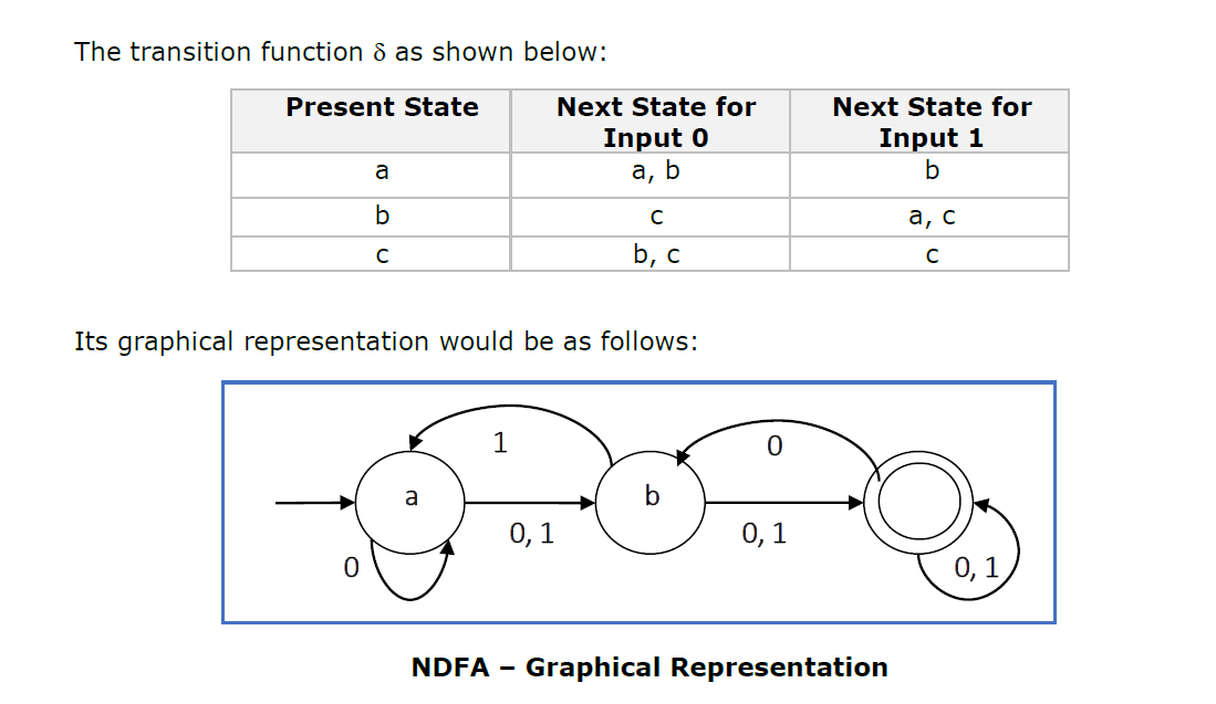
* δ is the transition function.
* q0 is the initial state from where any input is processed (q0 ∈ Q).
* F is a set of final state/states of Q (F ⊆ Q).

Alphabet
* Definition: An alphabet is any finite set of symbols.
* Example: Σ = {a, b, c, d} is an alphabet set where ‘a’, ‘b’, ‘c’, and ‘d’ are
symbols.

String
* Definition: A string is a finite sequence of symbols taken from Σ.
* Example: ‘cabcad’ is a valid string on the alphabet set Σ = {a, b, c, d}

Length of a String
* Definition : It is the number of symbols present in a string. (Denoted by |S|).
* Examples:
o If S=‘cabcad’, |S|= 6
o If |S|= 0, it is called an empty string (Denoted by λ or ε)

Kleene Star
 Definition: The Kleene star, Σ*, is a unary operator on a set of symbols or strings, Σ, that gives the infinite set of all possible strings of all possible lengths over Σ including λ.
 Representation: Σ* = Σ0 U Σ1 U Σ2 U……. where Σp is the set of all possible strings of length p.
 Example: If Σ = {a, b}, Σ*= {λ, a, b, aa, ab, ba, bb,………..}

Kleene Closure / Plus
* Definition: The set Σ+ is the infinite set of all possible strings of all possible lengths
over Σ excluding λ.
 Representation: Σ+ = Σ1 U Σ2 U Σ3 U…….
                           Σ+ = Σ* − { λ }
 Example: If Σ = { a, b } , Σ+ ={ a, b, aa, ab, ba, bb,………..}

Language
 Definition : A language is a subset of Σ* for some alphabet Σ. It can be finite or infinite.
 Example : If the language takes all possible strings of length 2 over Σ = {a, b}, then L = { ab, bb, ba, bb}

Time Complexity of Data Structure Operations

Big-O, Little-O, Theta, Omega

Big-O, Little-o, Omega, and Theta are formal notational methods for stating the growth of resource needs (efficiency and storage) of an algorithm. There are four basic notations used when describing resource needs. These are: O(f(n)), o(f(n)), $\Omega(f(n))$Ω(f(n)), and $\Theta(f(n))$Θ(f(n)). (Pronounced, Big-O, Little-O, Omega and Theta respectively)

• Big-O -- asymptotic upper bound (inclusive)
• little-o -- asymptotic upper bound (exclusive)
• Theta -- asymptotic tight bound (Big-O and Big-Omega)
• Big-Omega -- asymptotic lower bound (inclusive)

Best/worst/average case runtimes are specific values (can be asymptotic) that describe the shortest possible runtime, longest possible runtime, and expected runtime. 




Common Data Structure Operations

Data Structure	Time Complexity								Space Complexity
	Average				Worst				Worst
	Access	Search	Insertion	Deletion	Access	Search	Insertion	Deletion
Array	Θ(1)	Θ(n)	Θ(n)	Θ(n)	O(1)	O(n)	O(n)	O(n)	O(n)
Stack	Θ(n)	Θ(n)	Θ(1)	Θ(1)	O(n)	O(n)	O(1)	O(1)	O(n)
Queue	Θ(n)	Θ(n)	Θ(1)	Θ(1)	O(n)	O(n)	O(1)	O(1)	O(n)
Singly-Linked List	Θ(n)	Θ(n)	Θ(1)	Θ(1)	O(n)	O(n)	O(1)	O(1)	O(n)
Doubly-Linked List	Θ(n)	Θ(n)	Θ(1)	Θ(1)	O(n)	O(n)	O(1)	O(1)	O(n)
Skip List	Θ(log(n))	Θ(log(n))	Θ(log(n))	Θ(log(n))	O(n)	O(n)	O(n)	O(n)	O(n log(n))
Hash Table	N/A	Θ(1)	Θ(1)	Θ(1)	N/A	O(n)	O(n)	O(n)	O(n)
Binary Search Tree	Θ(log(n))	Θ(log(n))	Θ(log(n))	Θ(log(n))	O(n)	O(n)	O(n)	O(n)	O(n)
Cartesian Tree	N/A	Θ(log(n))	Θ(log(n))	Θ(log(n))	N/A	O(n)	O(n)	O(n)	O(n)
B-Tree	Θ(log(n))	Θ(log(n))	Θ(log(n))	Θ(log(n))	O(log(n))	O(log(n))	O(log(n))	O(log(n))	O(n)
Red-Black Tree	Θ(log(n))	Θ(log(n))	Θ(log(n))	Θ(log(n))	O(log(n))	O(log(n))	O(log(n))	O(log(n))	O(n)
Splay Tree	N/A	Θ(log(n))	Θ(log(n))	Θ(log(n))	N/A	O(log(n))	O(log(n))	O(log(n))	O(n)
AVL Tree	Θ(log(n))	Θ(log(n))	Θ(log(n))	Θ(log(n))	O(log(n))	O(log(n))	O(log(n))	O(log(n))	O(n)
KD Tree	Θ(log(n))	Θ(log(n))	Θ(log(n))	Θ(log(n))	O(n)	O(n)	O(n)	O(n)	O(n)

Array Sorting Algorithms

Algorithm	Time Complexity			Space Complexity
	Best	Average	Worst	Worst
Quicksort	Ω(n log(n))	Θ(n log(n))	O(n^2)	O(log(n))
Mergesort	Ω(n log(n))	Θ(n log(n))	O(n log(n))	O(n)
Timsort	Ω(n)	Θ(n log(n))	O(n log(n))	O(n)
Heapsort	Ω(n log(n))	Θ(n log(n))	O(n log(n))	O(1)
Bubble Sort	Ω(n)	Θ(n^2)	O(n^2)	O(1)
Insertion Sort	Ω(n)	Θ(n^2)	O(n^2)	O(1)
Selection Sort	Ω(n^2)	Θ(n^2)	O(n^2)	O(1)
Tree Sort	Ω(n log(n))	Θ(n log(n))	O(n^2)	O(n)
Shell Sort	Ω(n log(n))	Θ(n(log(n))^2)	O(n(log(n))^2)	O(1)
Bucket Sort	Ω(n+k)	Θ(n+k)	O(n^2)	O(n)
Radix Sort	Ω(nk)	Θ(nk)	O(nk)	O(n+k)
Counting Sort	Ω(n+k)	Θ(n+k)	O(n+k)	O(k)
Cubesort	Ω(n)	Θ(n log(n))	O(n log(n))	O(n)